Predicting building energy consumption with tensorflow
So, it is my first post so I probably should introduce myself briefly. I am currently studying in Loughborough University, UK under the London-Loughborough Centre for Doctoral Training in Energy Demand. Before that I did stuff in different industries mostly related to energy, in short. If you really are so interested, see my profile on LinkedIn or Twitter. Skip the next paragraphs if you want to just skip to the technical coding part.
One of the things that has struck me during these past years is the widening gap between applying computer science to other engineering disciplines. The simple reasons seems to be that computer science has progressed so rapidly that engineers haven’t been able to keep up. We do not really seem to know how to use the opportunities properly while computer science engineers do not know what to use their skills for. And we end up with this situation where our brightest minds and cutting edge technologies are used to maximizing the impact of internet ads… But let’s not go there now.
What I want to do is to bring computational techniques a bit closer to “real-life” and see how to realize their value and what could be a better application than energy-use with all its complexities. So more or less as a hobby I have been developing my hands-on skills in utilising different digital technologies and wish to share what I have been up to and hopefully share ideas with like-minded people.
First of all, I am a mechanical engineer by background without extensive background in coding so I apologies for all the messiness and errors which I will be making. As you will notice the approach is to get stuff work, instead of focusing on the nitty-gritty. I hope that this approach provides some value, especially for those who are (like me) not so into the “under-the-hood” things. Applications first!
Let’s get started. What I tried to do was to use a Python package called tensorflow for creating models for energy consumption of a building. I wanted to have a look at whether I could use tensorflow to create a simple trainable model for predicting energy consumption of a building by using outdoor temperatures. I basically followed the tensorflow tutorial structure but tweaked the code to better suit the energy domain. So really nothing revolutionary or advanced but definitely a start. A big thanks also to Arthur Juliani for his tutorials, they helped me a lot.
The full code and the files are available in github. My next plan will be to develop the code more modifiable and versatile. I also might try to create a learning controller by using Raspberry Pi3 along with tensorflow. I want to see how easy it would be to create an IoT device embedded with machine learning capabilities for the energy-specific domain. Feel free to contact if you have any inputs, critique, ideas or comments — I would be happy do discuss further!
Below is the main programme which calls the functions in pred_func.py during various stages. The workflow is pretty intuitive, first the data is handled, turned into inputs that tensorflow can use. The out-of-box estimators provided by tensorflow are then used to train two models, a linear regression model and a deep neural network with two hidden layers. After training the model is evaluated. Finally, outputs of the evaluations are also printed and plotted.
The main programme.
The pred_func.py defines the functions needed in the main programme. The read_data function reads the data from the csv-files and returns the testing and training data sets. The training and testing data is created from our original data by randomizing the data and then splitting it.
Functions train_tf and evaluate_tf are more interesting, they basically define the training and evaluation methods used. In tensorflow “features” is the input to our model, i.e. air temperature in this case. “Labels” are the outputs, gas consumption. In training data is shuffled, batched and used to map the input with the outputs. Evaluation works similar to training except that only features are input and then the model is used to predict the labels. For now the basic tensorflow methods are used to keep this straight-forward.
A cool feature of tensorflow is tensorboard which can be used to visualize the models created in tensorflow. Just modify the following code to point to your directory with the python files, run it and open the page https://your_hostname:6006 on your browser to check it out. It provides interesting visualizations regarding the structure and training of the models.
So, how did the models do? The DNN-model was run with a learning rate of 0.3, batch size was five for both models and regularizations were set to zero since I wanted to demonstrate the difference to traditional linear regression. Interestingly the DNN-model predicts a significant step-change in gas consumption temperatures are low and can thus provide such features for a data-driven modeller. If the underlying data were more interesting we might see more features in our model but since it was pretty straight-forward we only see this one major difference to the linear model.
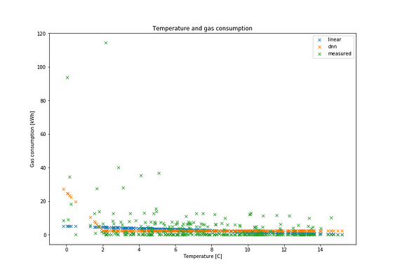
However, as is apparent from the figure, not much data existed for those very low temperatures and since regularization was set small the outliers can sway the model quite a lot and the models really are as good as was the data used to train them. Thus the results should be interpreted always with some skepticism, especially when data can be extremely noisy or hard to acquire as is typically the case with buildings.
We have built a very simple gas consumption predictor using tensorflow, so what? The point was to show that applications of AI and machine learning are not as far away as some might think. I believe these applications will also break-through to the energy sector where quantities of gathered data increase rapidly. This applies especially to the demand-side as it becomes an active component of the system.
This development is already driven forward by regulation which is making aggregation of flexible demand, real-time trading of energy and deeper integration of small-scale renewables increasingly common. I wish that these developments are used for the common good of us and the environment by creating a healthy energy system characterized by words like efficient, democratic and reliable. But equally machine-learning will probably have a role in any future scenario, also the more ominous ones.
From a practitioner to practitioners,
-Eramismus
This post was originally published in Medium
I am a practical Finn with interests spanning energy, digitalisation and society. I am currently working towards a PhD in England. Among other things I try to explore the layered nature of sustainability through philosophy and technology.