To flexineer, one needs to know where to start with. So far I have been exploring model-predictive control (MPC) and how to scalably characterise building energy demand with RC- and ARX-models. So, what have I found out? In this post I will briefly walk through my main findings from simulations and development of control strategies. The post is based on work that was also put in the form of an open-access paper in Applied Energy.

Control strategy

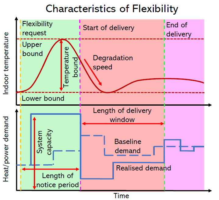
Contracted flexibility in its simple form means modifying heat demand, in our context, in exchange for a reward, ideally without reducing the level of service. For a reserve capacity service the most common request would be to reduce demand during pre-defined time windows in the morning when people wake up, say 7-8, and evenings when they arrive home and cook, 17-19.

To use MPC for this purpose the objective function has to somehow encapsulate this requirement. One could use a basic form of economic MPC where a time-varying price signal would be used to shape demand. But, flexibility for a reserve capacity service could also be a separate goal in the objective function to allow its delivery under varying energy pricing conditions and hence consider it at as a separate, even competing objective.

The objective function

So far, through pretty much trial and error I begun with testing various difference objective function formulations, both linear and non-linear. Below is the mathematical formulation which I found to best represent the behaviour I wish to achieve with the MPC.

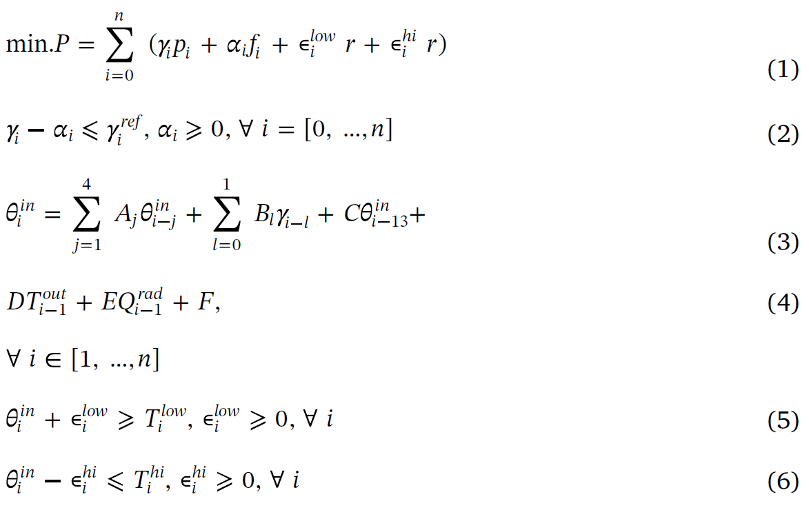
Let’s break it down a bit. The function (equation 1) is a sum of costs over a time horizon spanning n time-steps and the objective is to minimise that cost. Gamma is the control variable, i.e. heat demand. p is the price of electricity.

Alpha is the control variable for exceedances to a reference demand profile gamma-ref, which is what is activated by associating a cost f to times when there is a need to perform demand response. Otherwise, f is zero. The way it works, is that alpha is a decision variable which is either zero (no need to exceed the reference) or more than zero (the demand is exceeded). When it is more than zero, cost f is applied on to that exceedance. Epsilon-hi and epsilon-low are used in similar way to value comfort, i.e. deviations from a defined set point band, r is the cost for each violation to these bands.

ARX-models for predicting energy demand

Gamma is tied to the indoor air temperature through linear ARX-models (Auto-Regressive model with eXogenous inputs). The ARX-model structure is mathematically written with equations 3-4. The model structure was the same for all buildings, which was defined by evaluating a set of models with different parameter combinations, and chosen by using the best performing model structure on average over the community based on the Akaike Information Criterion (AIC).

In the MPC set up, gamma-ref is based on a demand projection of the MPC (gamma) one-time step before a call to modify demand, i.e. the projection with f set as zero. Gamma-ref is set by making a reduction request over the demand response window when f is set to some non-zero value.

Co-simulations of buildings

We now have our MPC, and to test it, I used co-simulations where the controller and buildings are simulated side-by-side. The method corresponds is emulating a situation where there would be a real building reacting to the actions of the controller.

In practice this I had my controller coded up in Python which then exchanged control decisions with JModelica.org, the simulation software that I use to emulate the real buildings. I used IBPSA single-zone Modelica models to represent the homes, in total 30 of them.

The point of co-simulation is to capture some of the reality a real controller would be facing, prediction errors, disturbances and uncertainty. For example, the demand projections the controller makes would in reality never be 100% accurate, which co-simulation can capture, as opposed to just simulating the controller operation.

Simulation cases

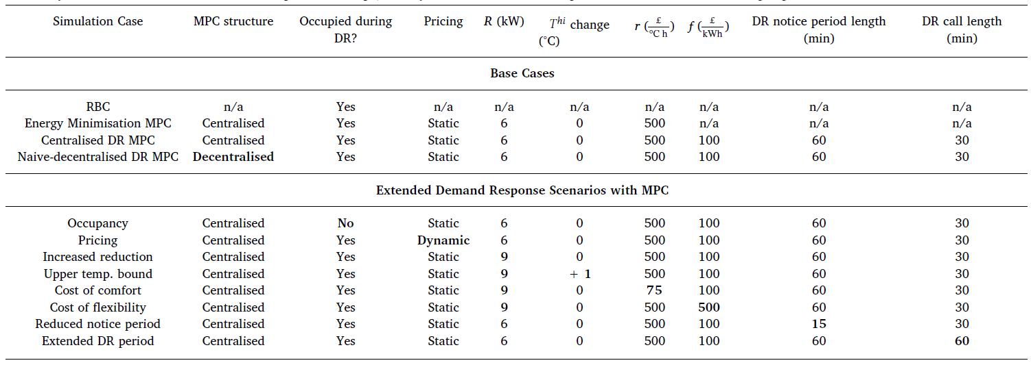
To explore the flexibility the MPC could provide with the building, a range of case studies was run to test different scenarios. The weather was varied by choosing three case days to represent winter, spring and autumn. For each case day demand response events were introduced over mornings and evenings, which is when the need for DR is typically at its high and electricity prices are high. The buildings were assumed to be occupied throughout the DR periods, one simulation was run with occupation ending before the DR window to illustrate effects of occupation on the flexibility potential.

To understand effects of the MPC structure, the MPC was run in decentralised and centralised modes. Simulations were run with different electricity prices p, a static fixed price and dynamic half-hourly pricing. Also other control parameters f and r were varied to show how costs allocated to flexibility or comfort would shift operation of the MPC and affect delivering the fixed demand reduction.

Table below illustrates the simulation case studies and what each case aims to observe and analyse:

Outcomes

By investigating the results from the simulation cases we built a comprehensive understanding of what characterises the contracted flexibility potential of a building, so-called factors of flexibility.

Below is a figure of how the centralised and decentralised MPC operated over mornings and afternoons in the three case days.

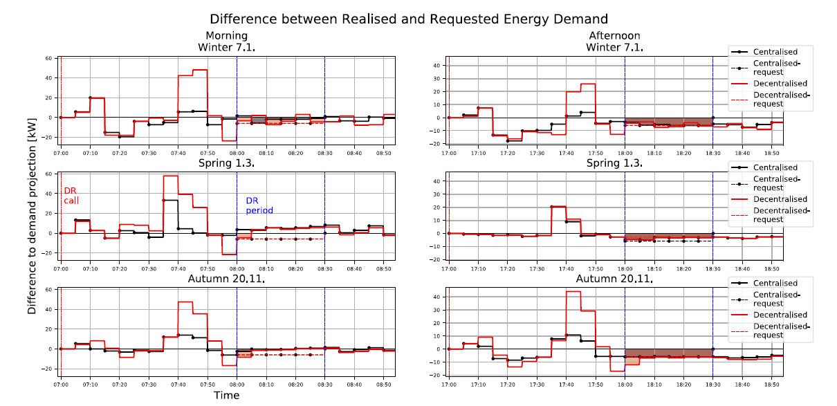
Let’s analyse this a bit. First of all, a predictive controller which has to maintain a set level of service will try to accommodate the DR request by preheating, where the building is heated before the DR period to minimise energy consumption during the DR period. It is like charging a battery, heat is consumed and “stored” to avoid its use later. The performance of the building and the community for this purpose thus depends on a number of factors.

Baseline challenge

The capability of a building in reality is not only determined by its physical ability to be act as storage but also in reality depends on the baseline energy demand, i.e. the benchmark used to define a demand modification. For a generator this benchmark would for example be a set level of power production. In the case of a building however establishing this baseline could be difficult given the variability in how energy is used in buildings and its dependence on dynamic factors like weather.

Factors of Flexibility

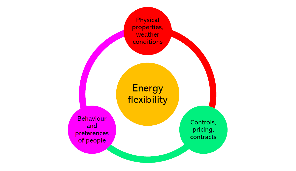
The contracted energy flexibility potential of a building, its ability to modify its energy consumption to fulfil a contract, is inherently dynamic due to the underlying drivers of energy use. The factors characterising this potential fall into three different categories:

1. Physical factors
2. Performance expectations
3. Market environment

The first refers to the physical interactions and conditions of the building, its systems and its environment. For example, its ability to retain heat, the weather, its HVAC systems and so forth.

The second, performance expectations, refers to the service requirements that the buildings needs to deliver. This element is dynamic, tiying the flexibility of the building to the way it is being used. For example in the case of homes, this means that the preferred indoor temperature and people’s comings and goings become important elements affecting the flexibility.

Finally, the market environment fundamentally defines the form of flexibility that is needed and how it is being incentivised. Depending on incentives, the ability to be flexible in return changes. If losses are weighed similarly to gains, this also applies in a counter-factual set up, where inflexibility would be penalised and being flexible would be to avoid a cost than to get an incentive.

Conclusions

Factors of flexibility, building’s physical characteristics, performance expectations and the market environment are intertwined and dependent, feeding into building energy flexibility. The building’s thermal behaviour is affected by its design which in turn are influenced by the market environment, intended use of the building and its users or occupants. The behaviour of people in a building does not occur in isolation, it is affected by the physical environment and their awareness of energy use and its costs, which is defined by the market. In case flexibility us voluntary, the willingness of people to participate is would be partly influenced by the incentives that the markets can provide and ease of participation.

Continuing the line of thought further leads to some interesting ideas. Flexibility could provide added value to energy efficiency investments. For example, a house with smarter, responsive controls and better ability to retain heat while being more efficient and comfortable, also enable other system-wide benefits.

However, before this can be verified, further research and development is needed to see whether schemes based on roll-out of smart controls in homes actually materialise and can replace peak power generation or other storage technologies.

To come: analysis of experiments over this winter.

-Eramismus

References

• El Geneidy, R., Howard, B. (2020). Contracted energy flexibility characteristics of communities: Analysis of a control strategy for demand response, In Applied Energy, Volume 263, 2020, 114600, ISSN 0306-2619, DOI: https://doi.org/10.1016/j.apenergy.2020.114600. URL: http://www.sciencedirect.com/science/article/pii/S0306261920301124.

• El Geneidy, R., & Howard, B. (2019). Delivery of Contracted Energy Flexibility from Communities. In Building Simulation 2019 - Rome, Italy. IBPSA. Retrieved from https://dspace.lboro.ac.uk/dspace-jspui/handle/2134/36405

• El Geneidy, R. S., & Howard, B. (2018). Review of techniques to enable community-scale demand response strategy design. USim2018 - Urban Energy Simulation. Retrieved from https://dspace.lboro.ac.uk/dspace-jspui/handle/2134/36259